Following on from last weeks post on plotting passes, I thought it might be fun to plot the shots and locations of players using the shot freeze frame in StatsBomb data. For those of you that haven’t already, I posted a tutorial around how to extract the freeze frame data included here. So if you need to, take a look at that post before going further.
For this post, I have loaded the following packages to use and colours to be applied to our plots further down:
library(tidyverse)
library(ggplot2)
library(ggsoccer)
library(ggrepel)

cols <- c("Arsenal WFC" = "red", "Manchester City WFC" = "blue",
          "Off T" = "yellow", "Post" = "orange", "Saved" = "green",
          "Blocked" = "grey")
I have loaded two data sources for this tutorial, my Freeze Frame data and also a summary of all the shots from the FA WSL. The reason for this is that the freeze frame doesn’t include the shot start and end location within it as the freeze frame is included in the event data itself. We will use this data to add detail to the shots and if they were crowded, or were open on target.
So let’s start with building our pitch again using ggsoccer. There will be one difference this week, in that we will rotate the pitch and only use one half.
pitchplot <- data %>%
  ggplot(aes(x=x, y=y)) +
  annotate_pitch(dimensions = pitch_statsbomb, colour = "white", fill   = "chartreuse4") +
  coord_flip(xlim = c(59,121), ylim = c(-1,81)) +
  theme_pitch() +
  theme(plot.background = element_rect(fill = "chartreuse4"),
        title = element_text(colour = "white"))

pitchplot
For this we used coord_flip to rotate the pitch, but this also flips our y co-ordinates as well, so will need to keep this in mind as we create our plots. So first up, let’s plot a shot, with it’s end location. For this we will use our shot summary (I have called this shotdata).
shotplot <- shotdata %>%
  filter(period == 1) %>%
  ggplot(aes(x=x, y=80-y)) +
  annotate_pitch(dimensions = pitch_statsbomb, colour = "white", fill   = "chartreuse4") +
  geom_point(aes(colour = shot.outcome.name)) +
  geom_segment(aes(x=x, y=80-y, xend=shot.end.x, yend=80-shot.end.y, colour = shot.outcome.name)) +
  scale_color_manual(values = cols) +
  coord_flip(xlim = c(59,121), ylim = c(-1,81)) +
  theme_pitch() +
  theme(plot.background = element_rect(fill = "chartreuse4"),
        title = element_text(colour = "white"))

shotplot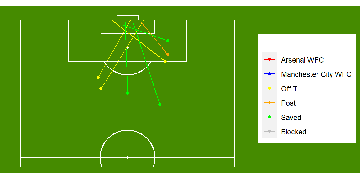
The first thing I will point out, is to account for our flipped y co-ordinates we needed to adjust our y values. In this context it is as easy as writing 80-y where we use our y values. This will correct their position on the pitch to be accurate. I have also used the outcome of the shot to colour the point and segment so we can add more context to the shot taken.
Now that we have the plot of shots, we are going to take one of these shots to plot the freeze frame as well. So let’s do that now:
freezedata <- data %>%
  filter(minute == 37)

freezeshotplot <- shotdata %>%
  filter(period == 1 & minute == 37) %>%
  ggplot(aes(x=x, y=80-y)) +
  annotate_pitch(dimensions = pitch_statsbomb, colour = "white", fill   = "chartreuse4") +
  geom_point(aes(colour = team.name), size = 2) +
  geom_segment(aes(x=x, y=80-y, xend=shot.end.x, yend=80-shot.end.y,
                   colour = shot.outcome.name), size = 1, alpha = 0.75) +
  geom_point(data = freezedata, aes(x=x, y=y, colour = `Team Name`)) +
  scale_color_manual(values = cols) +
  coord_flip(xlim = c(59,121), ylim = c(-1,81)) +
  theme_pitch() +
  theme(plot.background = element_rect(fill = "chartreuse4"),
        title = element_text(colour = "white"))

freezeshotplot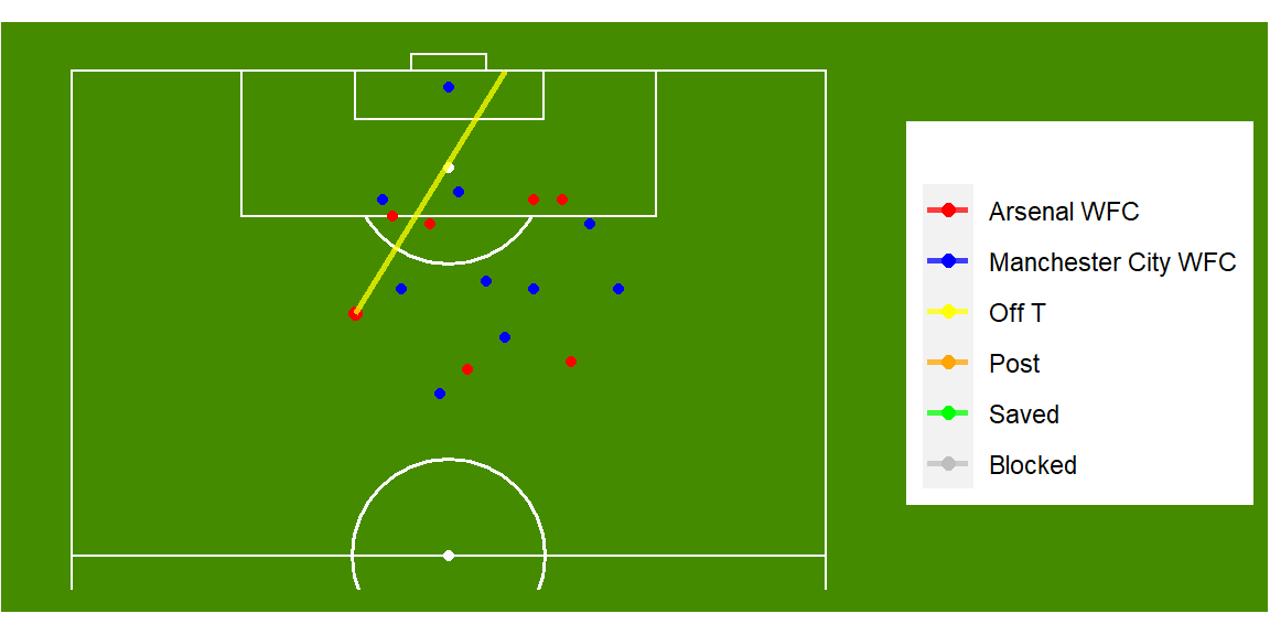
First, to make this plot possible I have filtered the freeze frame data to include the single shot we used from the summary data. I have then included added this as the data to our second geom_point call. I have then also included team name as a colour so that we can differentiate between teams. But I wonder if there is anything else we can add to this, for example, what would the xG be for a shot from this position on the pitch?
Let’s see:
freezexGshotplot <- shotdata %>%
  filter(period == 1 & minute == 37) %>%
  ggplot(aes(x=x, y=80-y)) +
  annotate_pitch(dimensions = pitch_statsbomb, colour = "white", fill   = "chartreuse4") +
  geom_point(aes(colour = team.name), size =2) +
  geom_segment(aes(x=x, y=80-y, xend=shot.end.x, yend=80-shot.end.y,
                   colour = shot.outcome.name), size = 1, alpha = 0.75) +
  geom_point(data = freezedata, aes(x=x, y=y, colour = `Team Name`), size = 2) +
  scale_color_manual(values=cols) +
  coord_flip(xlim = c(59,121), ylim = c(-1,81)) +
  theme_pitch() +
  theme(plot.background = element_rect(fill = "chartreuse4"),
        title = element_text(colour = "white")) +
  geom_label_repel(aes(label = round(shot.statsbomb_xg, 2),
                      fill = team.name,
                       size = 3.5),
                       colour = 'white') +
  theme(legend.position = "none")

freezexGshotplot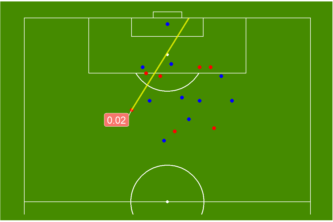
Now we have that, why don’t we add a text label so we know who took the shot and who they play for.
freezetextshotplot <- shotdata %>%
  filter(period == 1 & minute == 37) %>%
  ggplot(aes(x=x, y=80-y)) +
  annotate_pitch(dimensions = pitch_statsbomb, colour = "white", fill   = "chartreuse4") +
  geom_point(aes(colour = team.name), size =2) +
  geom_segment(aes(x=x, y=80-y, xend=shot.end.x, yend=80-shot.end.y,
                   colour = shot.outcome.name), size = 1, alpha = 0.75) +
  geom_point(data = freezedata, aes(x=x, y=y, colour = `Team Name`), size = 2) +
  scale_color_manual(values = cols) +
  coord_flip(xlim = c(59,121), ylim = c(-1,81)) +
  theme_pitch() +
  theme(plot.background = element_rect(fill = "chartreuse4"),
        title = element_text(colour = "white")) +
  geom_label_repel(aes(label = round(shot.statsbomb_xg, 2),
                       fill = team.name,
                       size = 2),
                       colour = 'white') +
  geom_label(aes(x=70, y=60, label = paste("Team: ", team.name), fill = team.name),
             colour = 'white') +
  geom_label(aes(x=65, y=60, label = paste("Player Name: ", player.name), fill = team.name),
             colour = 'white') +
  theme(legend.position = "none")

freezetextshotplot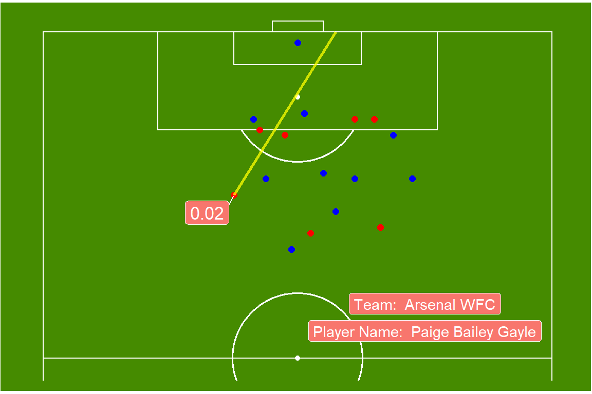
To add the labels, we used geom_label and geom_label_repel. Using ggrepel is a nice way of labels being forced to not overlap other points on the plot. To combine text and values from our dataset, we added values to a paste call, while using geom_label adds a nice background to the label. But let’s add even more detail by adding all the shots from a match by Arsenal. For this we wall call face_wrap in our plot creation.
matchfreeze <- data %>%
  filter(minute <= 45 & `Team Name.x` == "Arsenal WFC")

matchshotplot <- shotdata %>%
  filter(period == 1) %>%
  ggplot(aes(x=x, y=80-y)) +
  annotate_pitch(dimensions = pitch_statsbomb, colour = "white", fill   = "chartreuse4") +
  geom_point(aes(colour = team.name), size =2) +
  geom_segment(aes(x=x, y=80-y, xend=shot.end.x, yend=80-shot.end.y,
                   colour = shot.outcome.name), size = 1, alpha = 0.75) +
  geom_point(data = matchfreeze, aes(x=x, y=y, colour = `Team Name`), size = 2) +
  scale_color_manual(values = cols) +
  coord_flip(xlim = c(59,121), ylim = c(-1,81)) +
  theme_pitch() +
  theme(plot.background = element_rect(fill = "chartreuse4"),
        title = element_text(colour = "white")) +
  geom_label_repel(aes(label = round(shot.statsbomb_xg, 2),
                       fill = team.name,
                       size = 2),
                       colour = 'white') +
  geom_label(aes(x=70, y=60, label = paste("Team: ", team.name), fill = team.name),
             colour = 'white', size = 2) +
  geom_label(aes(x=65, y=60, label = paste("Player Name: ", player.name),
                 fill = team.name),
             colour = 'white', size = 2) +
  theme(legend.position = "none") +
  facet_wrap(~minute + second, ncol = 2)

matchshotplot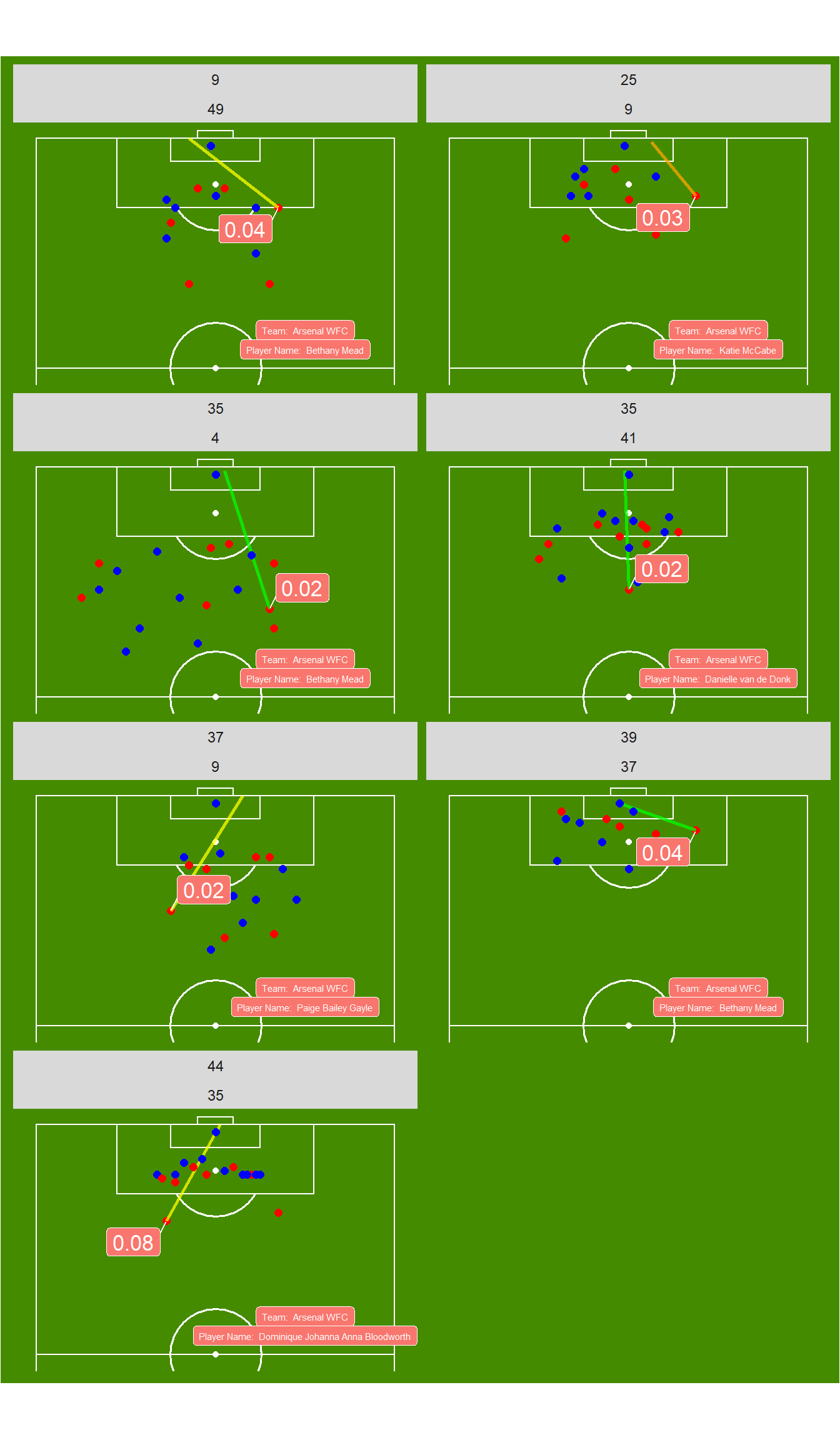
This plot shows all the shots from the first half of Arsenal vs Manchester City. From this we can see that Arsenal were unable to get in to good goal scoring positions. All their shots had below 10% chance of scoring, with most being off target. This can provide coaches are clear indication, if not already observed through footage, of where their team is shooting from and their probability of scoring from these positions. By including the freeze frame, it adds an extra level of detail, providing the position of all other players near the ball. Using this data we can add this to our expected goals model, strengthening the model overall, which is something missing from other models used currently.
This type of information is becoming more prevalent in football, with the inclusion of optical tracking the data obtained is even more powerful. StatsBomb are providing an incredible level of detail with the freeze frame data included in their match events, which is a real differentiator between them and other companies currently.
I hope you enjoyed this tutorial and feel free to contact me if you have any questions.
Thanks again to StatsBomb for the free data sources they provide!