Simple Shot Analysis

I was overwhelmed at the response and impressions on my first post that I decided to build on it sooner than expected. In today’s post I am going to look at a simple shot analysis in the FA Women’s Super League (FAWSL). In my last post I created a quick summary table of all the shots taken during the 2018-19 season, so we will use that to create a few simple plots and analyse a few shots in detail. To start with, let’s read in our data and find the top 6 scorers from the season. To do this, we will need to create a new column in our data, where the shot outcome is equal to goal. This will allow us to calculate goals easily using a sum function.

library(tidyverse)
library(ggsoccer)
library(ggplot2)

### Set the working directory before continuing.
### As this is in RMarkdown, I have done this earlier. 

HighestScorer <- Shots %>% 
  mutate(Goal = if_else(shot.outcome.name == "Goal", 1, 0)) %>% 
  group_by(player.name) %>% 
  summarise(Goals = sum(Goal))
HighestScorer <- HighestScorer[order(-HighestScorer$Goals),][1:6,]

player.name	Goals
Vivianne Miedema	37
Bethany England	23
Nikita Parris	19
Danielle van de Donk	16
Fara Williams	16
Georgia Stanway	15

Above, our tibble shows us who our top 6 scorers were from the StatsBomb data. Miedema and Parris scored 21 and 19 goals, respectively, which were quite easily the two top scorers during the season.

Now lets plot the Goals from our top 6 and see where they all came from on the pitch. First we will filter our main data set to only include players in the list above. Then we will filter out only the Goals scored during the season.

GoalsFilter <- Shots %>% 
  filter(player.name %in% HighestScorer$player.name) %>% 
  mutate(Goal = if_else(shot.outcome.name == "Goal", "1", "0"))

Goals <- GoalsFilter %>% 
  filter(Goal == "1")

ggplot(data = Goals, aes(x = x, y = y)) +
  annotate_pitch(dimensions = pitch_statsbomb, colour = "white", fill   = "chartreuse4") +
  geom_point(size = 2) +
  geom_segment(aes(x = x, xend = shot.end.x, y = y, yend = shot.end.y), size = 1) +
  coord_flip(xlim = c(59, 121),
             ylim = c(-1, 81)) +
  facet_wrap(~player.name) +
  theme_pitch() +
  theme(plot.background = element_rect(fill = "chartreuse4"),
        title = element_text(colour = "white")) +
  theme(legend.position = "top", legend.title = element_blank())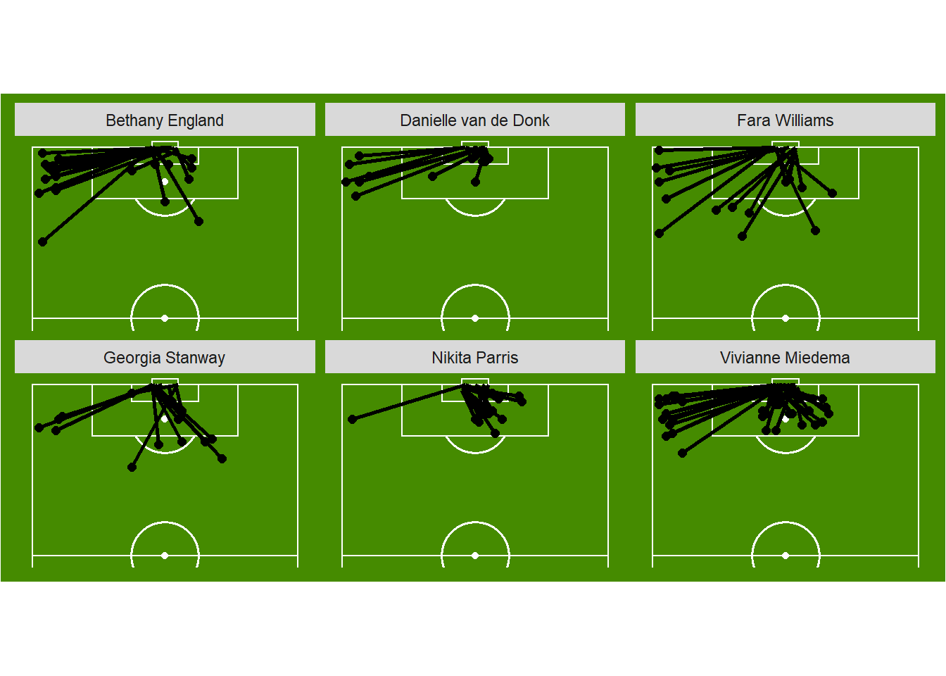

We can see from this plot, most of the goals scored were inside the box compared to outside. However, it looks like Fara Williams can is quite proficient from outside the box, so it makes you wonder how she scored. Did these goals come from open play or were they free kicks, lets take a deeper look in to her goals. First, let’s look at what foot she used to score her goals.

FaraGoals <- Goals %>% 
  filter(player.name == "Fara Williams")

ggplot(data = FaraGoals, aes(x = x, y = y)) +
  annotate_pitch(dimensions = pitch_statsbomb, colour = "white", fill   = "chartreuse4") +
  geom_point(size = 2, aes(color = shot.body_part.name)) +
  geom_segment(aes(x = x, xend = shot.end.x, y = y, yend = shot.end.y, color = shot.body_part.name), size = 1) +
  coord_flip(xlim = c(59, 121),
             ylim = c(-1, 81)) +
  facet_wrap(~player.name) +
  theme_pitch() +
  theme(plot.background = element_rect(fill = "chartreuse4"),
        title = element_text(colour = "white")) +
  theme(legend.position = "top", legend.title = element_blank())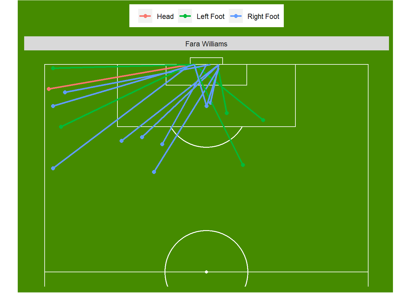

We can see in the above plot, she scored most of her goals with her right foot from the left hand side of the pitch. Being a central midfielder and considered a set-piece specialist, let’s see how many of these goals were from set-pieces, open play or penalties.

GoalDist <- FaraGoals %>% 
  filter(shot.type.name == "Free Kick")

ggplot(data = FaraGoals, aes(x = x, y = y)) +
  annotate_pitch(dimensions = pitch_statsbomb, colour = "white", fill   = "chartreuse4") +
  geom_point(size = 2, aes(color = shot.type.name)) +
  geom_segment(aes(x = x, xend = shot.end.x, y = y, yend = shot.end.y, color = shot.type.name), size = 1) +
  coord_flip(xlim = c(59, 121),
             ylim = c(-1, 81)) +
  facet_wrap(~player.name) +
  theme_pitch() +
  theme(plot.background = element_rect(fill = "chartreuse4"),
        title = element_text(colour = "white")) +
  theme(legend.position = "top", legend.title = element_blank()) +
  geom_label(data = GoalDist, label = paste(round(GoalDist$DistToGoal), "m"), nudge_x = -3)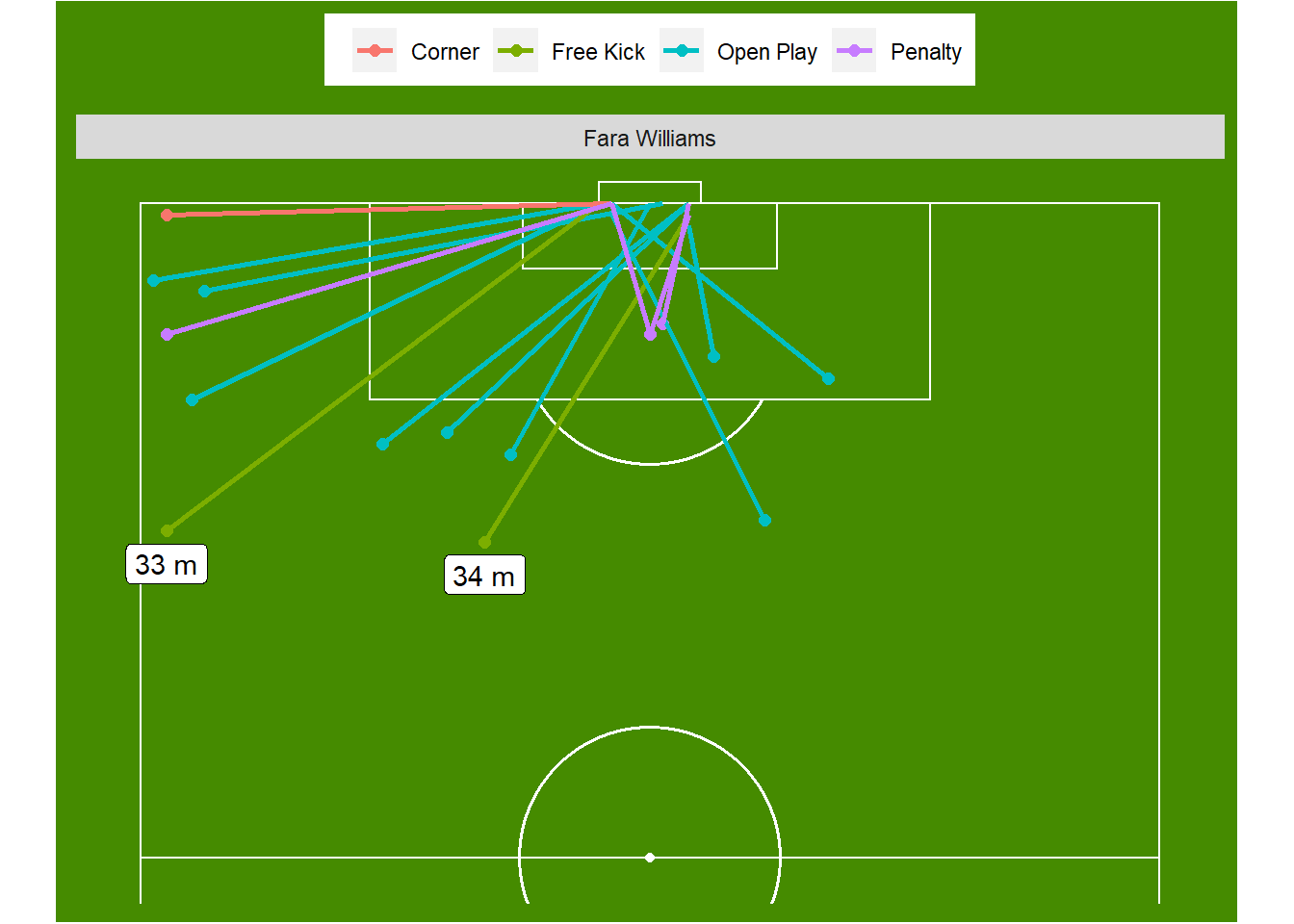

It’s interesting to see she only scored one goal from a free kick, with most of her goals coming from open play, showing the difficulty of scoring from set-piece situations. But that one free kick did come from 34 m away from goal, which shows the skill she must have. This is only a very simple analysis, but can show you the power of R and the free StatsBomb data. We can profile players on any number of things, to provide an data based overview of a players ability. In the age of data, this is can provide a replacement for scouts in some situations.

If you would like the full code, or have any questions, don’t hesitate to contact me. I will endeavor to get back to you all quickly.

Hope you all enjoyed this quick little analysis of goals scored in this seasons FAWSL. Look forward to digging further in to this data soon!